
What should
we quote?
Change the market. Set a price. Reveal the result. Then test how quickly the calculation runs.
INFORMATION → QUOTE → OUTCOME
A fill is only useful
at the right price.
Read a noisy market. Price the risk of being right on the fill
and wrong on the next price move.
Dealer sells one unit
5-second markout · values in bps
The market before the quote
The filter sees two noisy signals and their history. The hidden state and future outcome are withheld.
Your sell quote
above midpoint
Per RFQ, after costs and inventory penalty
More fills. Or better fills.
Better information changes the decision. Reusing calculations makes it faster.
Better decisions.
Faster calculation.
Two separate questions, measured separately.
Risk-adjusted bps per RFQ. Same optimiser, costs and inventory. 2,000 held-out synthetic RFQs.
How certain is that result?
Known model, one seed. The split is 3,000 training, 1,000 validation and 2,000 test RFQs. Inventories are independent snapshots. These are one-step marked values, not a trading P&L.
Calculate once.
Reuse for each quote.
Against 1,024-panel reference integration on the held-out test. This measures numerical agreement within the model.
What does the timer include?
Each method runs in a fresh CPU worker. One batch filters 128 RFQs, scans 41 quotes for each, and selects the best action. Cold timing includes table preparation. Nine warm batches follow a warmup.
The comparison uses 64-panel direct and precomputed integration. The displayed time is the median batch time divided by 128. It excludes input decoding, module loading, rendering and network time. It is not an individual request latency guarantee.
Where does quantum fit?
The working demo runs on a classical CPU. The next experiment would compare simulated quantum features with strong classical and random features on the same chronological data splits.
Implemented, proposed and still unknown
Implemented Synthetic market, causal Bayesian filter, inventory-aware quotes and measured CPU precomputation.
Proposed Quantum feature experiments and NVIDIA GPU benchmarks. Neither is executed by this demo.
The HSBC–IBM paper motivates offline feature generation followed by fast inference. Its reported AUC results do not establish trading profit or quantum advantage. Hardware-noise and possible processing-order effects remain unresolved.
Read the HSBC–IBM study ↗When should a solver
reuse, refine or rebuild?
Finn Smith · Discussion draft · 27 October 2026
The proposal studies adaptive precision, iterative refinement and factorisation refresh for changing sparse/KKT systems.
This quote demo reuses scalar integration moments. It does not implement or validate the proposal’s solver. A future constrained quote or hedge problem could provide related KKT systems, but that formulation and its performance still need testing.
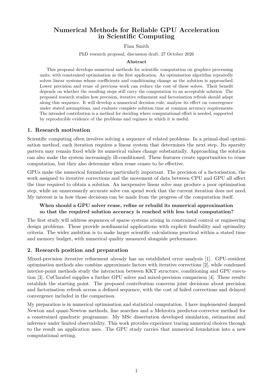
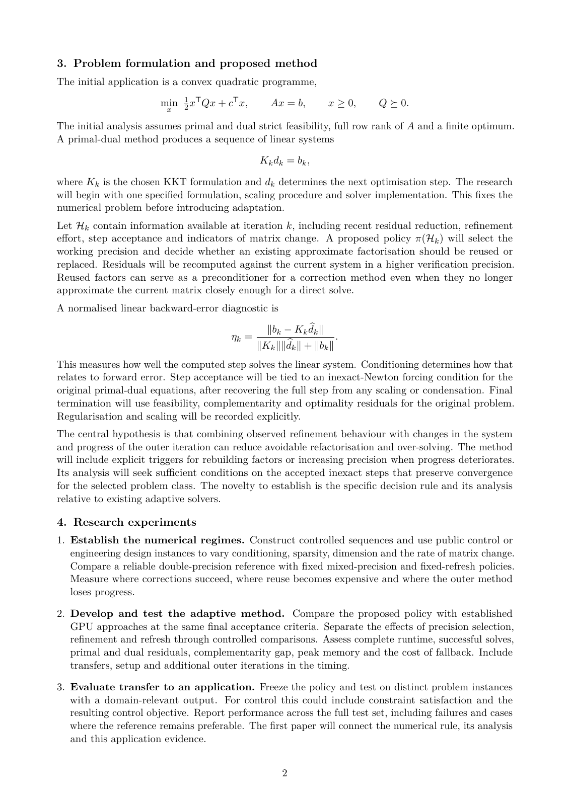
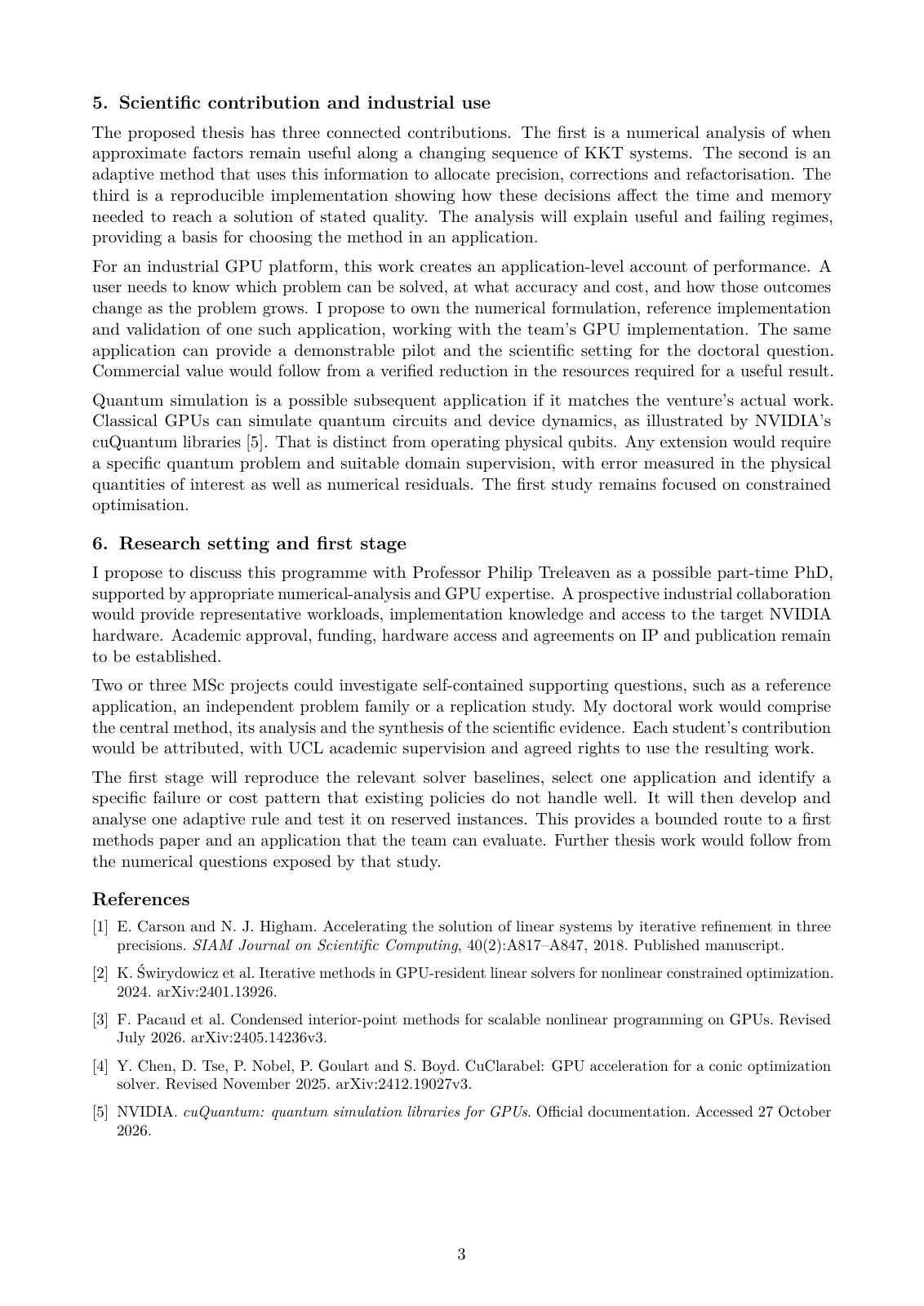
Read the original three-page proposal
Pinch to zoom the pages, or open the original PDF below.
TWO QUESTIONS. TWO SEPARATE TESTS.
Does it help?
Does it compute faster?
A locked chronological test and a calculation you can rerun.
The same market, different decisions
Expected values use hidden simulation truth only in evaluation. Realised values use the same random shocks for every policy. Inventory is a sequence of independent snapshots, so these are one-step marked values, not a trading P&L.
A fairer baseline
State blind uses the same quote optimiser, costs and inventory. It only omits the two signals. The fixed quote is selected on training outcomes.
Sampling uncertainty
Calibration at a common quote
Do the expensive part once.
Error compares cached decisions with 1,024-panel fresh integration on every held-out RFQ. It measures numerical agreement within this model. It does not measure market predictability.
The speedup comes from avoiding repeated integrals on the CPU.
THE MODEL AND ITS BOUNDARIES
Every claim has
a place in the experiment.
A small, reproducible decision problem with room to grow.
No live market connection
No orders or private data
A deliberately bounded market
A client asks to buy one unit. The dealer can sell from 0.0 to 4.0 bps above midpoint in 0.1 bp steps, or decline. A persistent hidden state takes the values −1, 0 or +1.
Two noisy signals feed a causal three-state Bayesian filter. Parameters are specified and known. They are not learned from market data. The filter uses these signals only, not information in past midpoint changes.
Inspect the equations
x = z + 1.15 ε₁
f = 0.7z + ε₂
P(fill | z, e, δ) = sigmoid(1.7 − 1.15δ + 0.9z + 0.9e)
Δm = 1.5z + 0.65e + 0.65ε₃
c(q) = 0.16 + 0.04|q − 1|
ΔR(q) = 0.12[(q − 1)² − q²]
V(δ) = E[fill × (δ − Δm − c(q) − ΔR(q)) | observed signals]
All ε and e are independent standard normals before selection. The shared private shock e makes accepted trades more adverse. Inventory q is an independently sampled integer from −3 to +3.
The state transition rows are [0.94, 0.06, 0], [0.03, 0.94, 0.03] and [0, 0.06, 0.94]. Initial probabilities are [0.25, 0.5, 0.25].
Why precomputation works
For each state and quote, save A = E[fill] and B = E[fill × Δm]. Then compute V = Σ p(z)[A(δ − c − ΔR) − B]. The online decision needs only the new posterior and current inventory.
Composite Simpson integration uses [−9, 9] for the private normal shock. The omitted probability is below 2.3 × 10⁻¹⁹. Validation selects the first grid with value error below 10⁻⁷ bps and no changed decisions. The quote grid is discrete, not a claim of a continuous optimum.
A chronological experiment
3,000VALIDATE
1,000TEST
2,000
Training chooses a fixed quote. Validation chooses the integration resolution. The held-out test is used once to report decisions and numerical error. The filter carries forward its state using observations available at each time.
RFQs arrive every 10 seconds. The markout occurs 5 seconds after each quote. Future state, private shocks, fills and markouts never enter the policy inputs.
What this experiment cannot establish
The model is stationary and correctly specified. There is no competition feedback, empirical bond calibration, queue model, dynamic hedging strategy or execution infrastructure. The outcome horizon and inventory penalty are chosen for this demonstration.
The expected gain is specific to this synthetic model. The block bootstrap describes sample variability, not uncertainty about model misspecification. Brier scores across different chosen quotes are not a fair ranking of predictors, so the calibration comparison fixes the same quote.
The quantum question stays open.
The HSBC–IBM study motivates separating offline feature generation from online inference. Section 4.2 reports AUC uplifts on its private bond data, with weaker noiseless-simulation results and unexplained hardware-noise effects. Processing order and possible label leakage remain concerns. Section 4.3 explores reuse through event matching.
That result is not a profit result or established quantum advantage. This application does not reproduce their dataset, circuit or hardware result.
Next experiment Add a small, deterministic circuit simulator. Compare its features with a strong classical filter, nonlinear features and equal-size random features on identical chronological splits. Report calibration, decision value and total feature-generation cost, including negative results.
Read HSBC–IBM, including §§4.2–4.3 ↗Scale the workload before the claim.
The current experiment runs on CPU. The saved benchmark records an Apple M1 Max. There is no NVIDIA benchmark or physical quantum processor result.
Benchmark contract Batch 128, 1,024 and 16,384 independent state and quote scenarios. Compare a vectorised CPU reference, precomputed CPU moments and an NVIDIA implementation at equal decision accuracy. Include initialisation, transfers, precision and memory use. Synchronise device work before timing.
For quantum simulation, use cuQuantum or CUDA-Q only on an authorised NVIDIA resource. GPU circuit simulation and a physical QPU are different computations.
cuQuantum ↗CUDA-Q ↗Useful connections, distinct models
01 Optimal Quoting under Adverse Selection and Price Reading Quote choice and informational risk ↗02 Hawkes-Driven OTC Market Making Persistent request flow and numerical approximation ↗03 Unwinding Toxic Flow with Partial Information Inference, inventory and hedging ↗04 JaxMARL-HFT GPU simulation at a different scale ↗05 CuClarabel GPU optimisation with accuracy checks ↗These sources inform the research context. Their algorithms and empirical results are not implemented or reproduced here.
RESEARCH PROPOSAL · DISCUSSION DRAFT
Reliable GPU acceleration.
A numerical research question.
Finn Smith · 27 October 2026 · Original three-page proposal
How this application connects
Reusable RFQ moments
A three-state filter and 41-quote grid combine precomputed Simpson integrals on CPU. The experiment tests decision value and numerical agreement.
Adaptive sparse/KKT solves
Choose precision, iterative corrections and factorisation refresh along a changing system sequence. Evaluate complete time at common feasibility and optimality requirements.
The RFQ demonstration is a numerical application. It does not implement, validate or establish novelty for the proposal’s adaptive solver.
A possible finance application
A future constrained quote or hedge optimisation could generate related KKT systems. That would provide a place to test the proposed reuse and precision policy against a reliable reference, including transfers, failed corrections and extra outer iterations.
The current one-step quote scan forms no KKT system. Any extension needs an explicit formulation and evidence at matched final accuracy. The proposal’s first study remains focused on constrained control or engineering problems.
Numerical Methods for Reliable GPU Acceleration in Scientific Computing
Research proposal and discussion draft, not a completed doctoral thesis. The PDF is reproduced unchanged. Pinch to zoom on a phone.